There was a quiet excitement in the air when we were using standard RNNs to make sense of sequential data in the early 1990s. In theory, these networks were elegant. They were supposed to keep track of their internal state as they moved through a sequence, remembering what came before. It sounded almost like a person; the model seemed capable of remembering the past while reading the present. But the real world hit different; these RNNs were surprisingly forgetful in real life. When they were demonstrated, something strange would happen as information moved through long chains of inputs: the gradient would either fade away or explode out of control. The beginning was completely erased by the time the network got to the end of a lengthy sentence; it was as if it had never existed.

In 1997, however, a big change happened. Jürgen Schmidhuber, a German computer scientist, wrote a paper called Long Short-Term Memory that quietly changed the future of sequence modeling. The idea was both simple and deep: make a path through time that could keep information safe instead of letting it fade away. This new architecture had well-planned feedback loops that let gradients flow steadily across many time steps instead of disappearing into silence. For the first time, a network could really remember things, holding on to the past while learning from the present.

LSTM (Long Short-Term Memory)

The ideal architecture of LSTM is as follows:

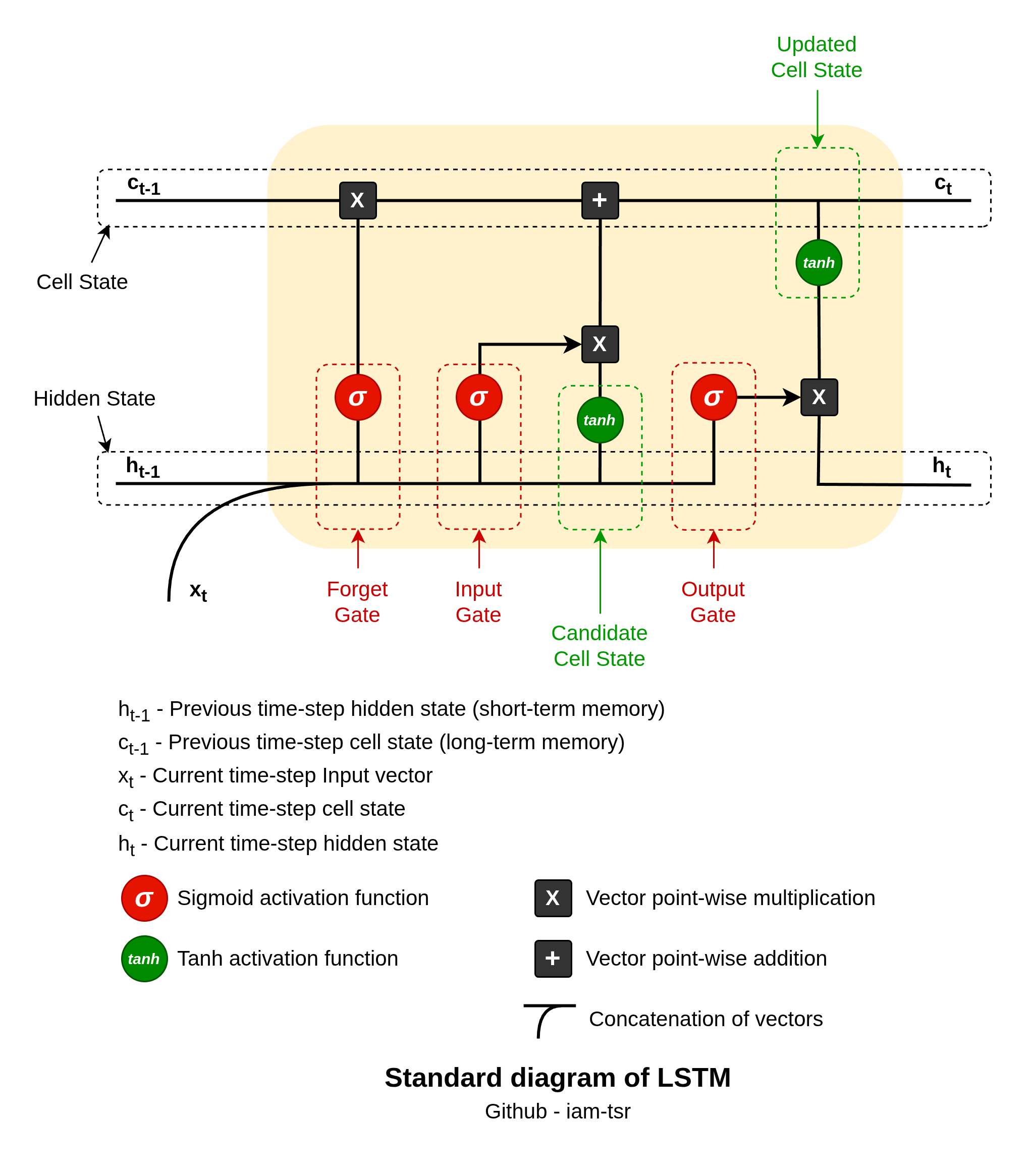
LSTM cells feature three gates: forget, input, and output — plus a candidate cell state. All of these are implemented as neural network layers with sigmoid $(\sigma )$ or $tanh$ activations. These gates control how the cell state changes by using element-wise operations $(\odot )$. You can see this as a “Cell State” flow, with previous states coming in from the left, gates crossing the path, and outputs going out to the right. The “Updated Cell State” mentioned in the image performs element-wise multiplication with the output gate to form a new hidden state (short-term memory). It used gating mechanisms to control the flow of information over long sequences. This strategy solved the problem of simple RNNs’ vanishing gradients.

Step by step flow

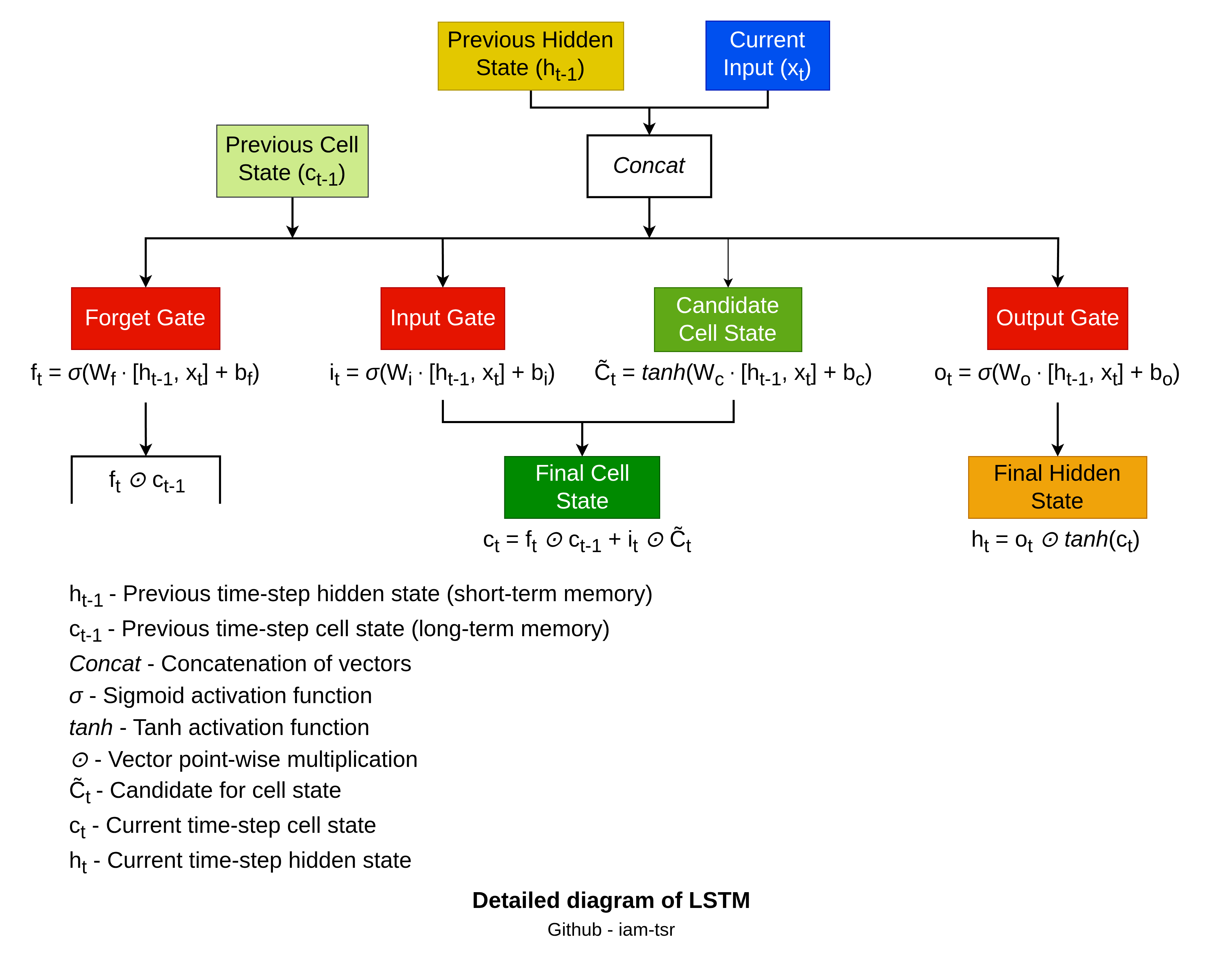
The process follows a fixed sequence per time step:

• Forget Gate: This gate decides what to discard from the previous cell state $(c_{t-1})$, preventing irrelevant info buildup. It concatenates previous hidden state vector $(h_{t-1})$ and current input vector $(x_t)$, applies weights $(W_f)$ and bias $(b_f)$, then sigmoid $(\sigma )$ for values in:

  $f_t=\sigma (W_f[h_{t-1},x_t]+b_f)$

  Here, $f_t$ multiplies $c_{t-1}$ element-wise: $f_t\odot c_{t-1}$, forgetting irrelevant info (1 keeps, 0 forgets). Learned via back propagation to drop outdated patterns, aiding gradient flow.

• Input Gate: Controls new information addition to $c_t$.

  Two steps: sigmoid gate $i_t=\sigma (W_i[h_{t-1},x_t]+b_i)$ filters relevance; $tanh$ creates candidate ${\tilde{C}}_t=tanh(W_c[h_{t-1},x_t]+b_c)$ bounded $[-1,1]$. Combined: $i_t\odot {\tilde{C}}_t$ adds selectively: $c_t=f_t\odot c_{t-1}+i_t\odot {\tilde{C}}_t$. Balances old retention with fresh updates.

• Candidate Cell State: It is not a gate but the $tanh$ proposal for new memory values, using same inputs as input gate. It provides bounded updates (prevents explosion) added via the input gate’s scaling. Acts as ‘new info vector’ injected into the linear cell state path.

• Output Gate: Filters updated $c_t$ for next hidden state $h_t$, which carries short-term info forward. Sigmoid: $o_t=\sigma (W_o[h_{t-1},x_t]+b_o)$; $tanh$ normalizes $c_t$: $h_t=o_t\odot tanh(c_t)$

  Exposes only relevant cell parts downstream, decoupling long-term storage from immediate output.

Cell state flows additively (minimal changes for long dependencies); gates multiply along paths, learned end-to-end. All use shared inputs for context-aware decisions.

My Life Is Going On

You might remember that title from somewhere. Take a moment to think about it. That one, yes. La Casa De Papel’s intro BGM. A return that seemed unnecessary at first but somehow had to happen. Another heist in the series wasn’t about desire, it was about necessity.

There was a moment like that in deep learning too. LSTMs had already fixed the problem of simple RNNs forgetting things. They could remember things for a long time, like vault secrets. But they came with weight. Multiple gates, separate cell states, more parameters, heavier computation. Yes, powerful. Not always efficient.

So the question came up. How? How to get around these issues?

Kyunghyun Cho, Yoshua Bengio, and their team came up with the GRU (Gated Recurrent Unit), in 2014. It wasn’t meant to beat LSTM in every situation. It was made to make it easier. GRU combined the forget and input gates into one update gate and the cell state with the hidden state. Fewer gates, fewer parameters, less computational overhead.

LSTMs are great at modeling long-term dependencies, but they can be complex to understand and take longer to train. GRUs became the better choice because they were faster to compute, easier to train, and just as effective. Not a replacement, but a refinement.

Why GRUs were developed and are necessary

• Two Gates vs. Three: LSTMs require managing three gates (input, forget, output) and a hidden/cell state, while GRUs only use two (reset and update). This makes them easier to implement and modify.
• Fewer Parameters: GRUs combine the input and forget gates of an LSTM into a single ‘update gate’ and merge the cell state and hidden state. This reduction in components results in roughly 25% fewer parameters, allowing for faster training and reduced memory consumption.
• Faster Training Speed: Because of their simpler architecture, GRUs are generally faster to train and run inference on than LSTMs, making them ideal for real-time applications or when working with limited computational resources.

GRU (Gated Recurrent Unit)

The ideal architecture of GRU is as follows:

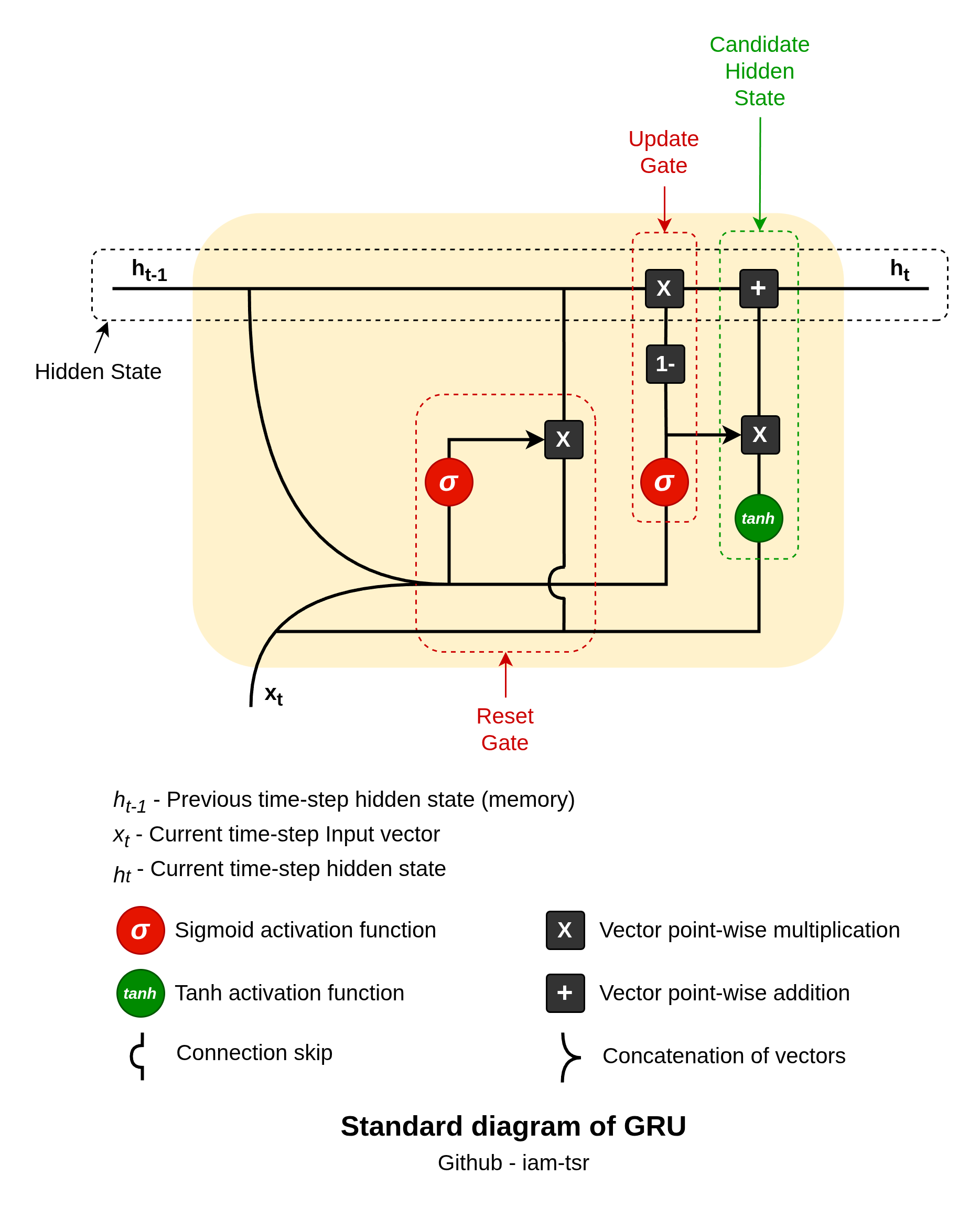
GRU cell features two key gates — update and reset — to selectively retain or discard information, making them computationally lighter than LSTMs.

Step by step flow

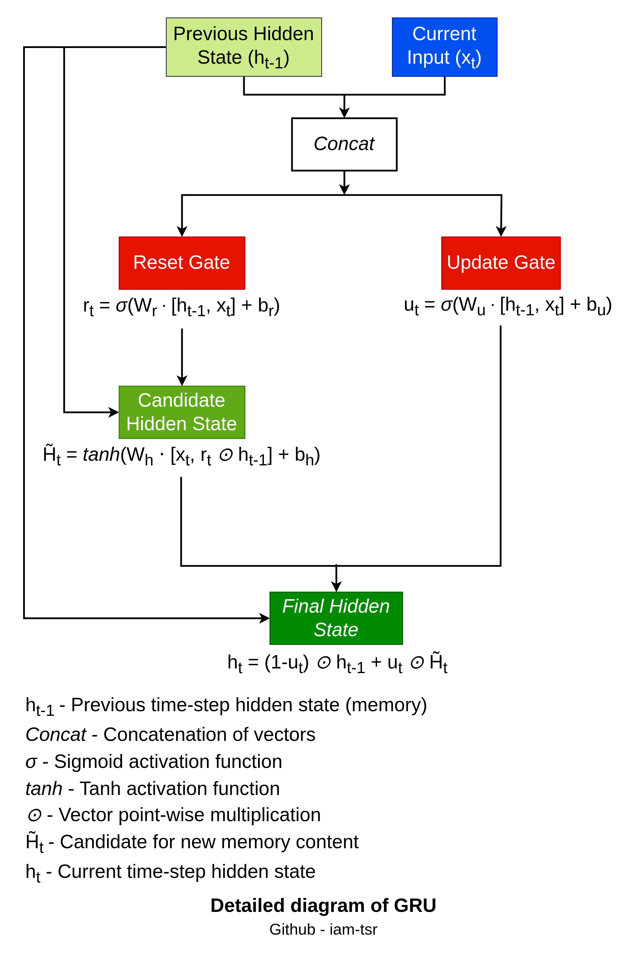
The GRU update follows these steps:

• Reset Gate: $r_t=\sigma (W_r[h_{t-1},x_t]+b_r)$. This decides how much of $h_{t-1}$ to forget when computing the candidate state (1 = keep all, 0 = ignore past).
• Update Gate: $u_t=\sigma (W_u[h_{t-1},x_t]+b_u)$. This balances old and new information (1 = fully update, 0 = retain old state).
• Candidate Hidden State: ${\tilde{H}}_t=tanh(W_h\cdot [x_t,r_t\odot h_{t-1}]+b_h)$, where ⊙ is element-wise multiplication. The reset gate filters $h_{t-1}$ before $tanh$ non-linearity.
• Final Hidden State: $h_t=(1-u_t)\odot h_{t-1}+u_t\odot {\tilde{H}}_t$. This interpolates between previous and candidate states.

The fall of all RNN types

LSTM (Long Short-Term Memory) and GRU (Gated Recurrent Unit) networks were designed to solve the vanishing gradient problem of simple RNNs; however, despite their gating mechanisms, they still struggle with very long-term dependencies, such as remembering information from 1,000 steps ago.

The main challenge with LSTM & GRU was that they cannot process the entire sequence at once; they cannot take full advantage of modern GPU hardware. They process data sequentially, one time step at a time. The hidden state of the current step depends on the calculation of the previous step, which leads to significantly slower training and generation times.

Despite this, they continue to be effective tools for processing sequential data. However, due to critical limitations in efficiency, parallelization, and handling extremely long-range dependencies, they have largely lost their relevance in many state-of-the-art applications.

---

The story is not finished yet. Isn’t it? We will see what happened when the golden age came in 2017 with a paper proposed by Google — “Attention is all you need.” Yes, in the next blog, we will learn about Transformers. Until then, keep shaping yourself!