So far, we've built the foundation step by step. First, we saw how raw text is broken down into smaller chunks called tokens, and then how those tokens are converted into vectors that a model can understand. Along the way, we explored two essential building blocks: token embeddings, which capture the meaning of each token, and positional embeddings, which tell the model where each token appears in the sequence. By combining these two embeddings, we create the input embeddings that are fed into the heart of the Transformer architecture.

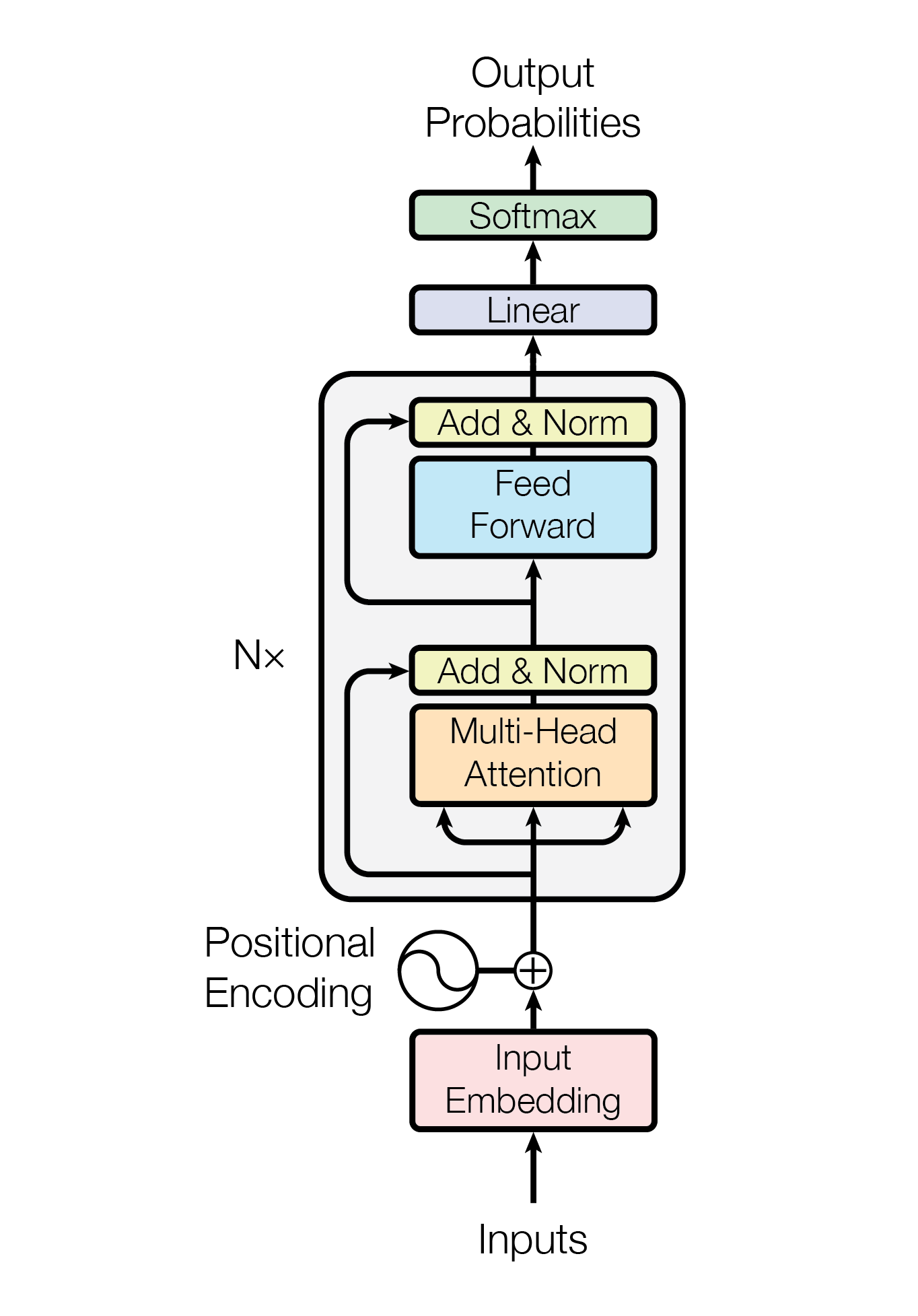
With that foundation in place, it's time to focus on encoder-only Transformers. The original Attention Is All You Need paper introduces the attention mechanism first, but over time, different Transformer architectures have adapted attention in different ways depending on their purpose. Since our focus is encoder-only Transformers, let's explore the specific attention mechanism they rely on and see how it fits into the overall architecture.

Types of Attention:

Self Attention:

Now that our input embeddings are ready, we can finally reach the heart of the Transformer—the self-attention mechanism. This is the mechanism that allows every token in a sentence to look at every other token and decide which ones are most relevant when building its representation.

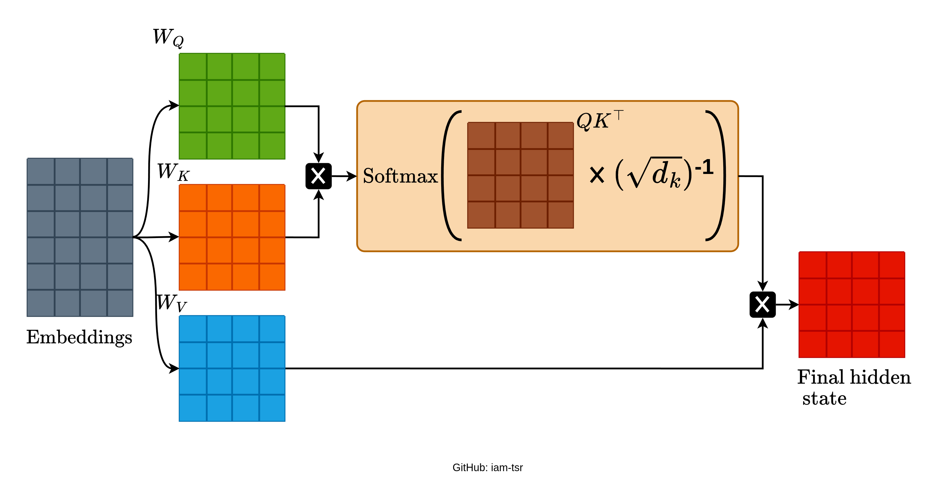
The first step is to generate three different representations for every input token: Queries (Q), Keys (K), and Values (V). These are computed by multiplying the input embeddings with three separate learnable weight matrices.

$$\begin{gathered} Q=X{W}^Q \\ K=X{W}^K \\ V=X{W}^V \end{gathered}$$

where:
$Q$ (Query): Represents what a token is looking for.
$K$ (Key): Represents what information each token has available.
$V$ (Value): Represents the actual information carried by each token.
$X$: The input embeddings, typically represented as a 3-dimensional tensor with shape $[batchsize,sequencelength,hiddendimension]$.

Let's use the sentence: $\text{"Aryabhata invented the concept of zero."}$

(We'll keep this sentence only to understand the mathematics. If you haven't read Part 1, that's perfectly fine—we'll skip the tokenization process and begin directly from the embeddings.)

Using BERT as an example, each token is converted into a 768-dimensional embedding.

• $\text{Aryabhata}-[0.2154,0.5478,\mathrm{0.5487...}765morevalues]$
• $\text{invented}-[0.7879,0.5748,\mathrm{0.6875...}765morevalues]$
• $\text{the}-[0.5648,0.5478,\mathrm{0.5787...}765morevalues]$
• $\text{concept}-[0.5475,0.5788,\mathrm{0.5479...}765morevalues]$
• $\text{of}-[0.46478,0.4876,\mathrm{0.4684...}765morevalues]$
• $\text{zero}-[0.5748,0.5789,\mathrm{0.5768...}765morevalues]$

Since we have a single sentence with five tokens, our input tensor has the shape:

• Batch size = $1$
• Sequence length = $6$
• Hidden dimension = $768$

So the input embeddings have the shape: $[1,6,768]$.

When training a Transformer from scratch, the matrices $W^Q$, $W^K$ are initialized randomly. Because they are learnable parameters, the model continuously updates them during training until they capture meaningful relationships between tokens.

Once these matrices are learned, every input embedding is projected into its corresponding Query, Key, and Value representations by multiplying it with $W^Q$, $W^K$, and $W^V$, respectively.

With the Query, Key, and Value matrices ready, we can compute the Scaled Dot-Product Attention, which lies at the core of every Transformer.

$$\mathrm{Attention}(Q,K,V)=\mathrm{softmax}\left(\frac{Q{K}^{\top }}{\sqrt{d_k}}\right)V$$

Where:

• $(K^T)$ is the transpose of the Key matrix.
• $(\sqrt{d_k})$ is the dimension of the Key vectors.
• $(\mathrm{softmax})$ converts the attention scores into probabilities so that every row sums to 1.

FAQ

Q. Why do we divide by ($\sqrt{d_k}$)?

Imagine calculating the dot product between two very large vectors. As their dimension increases, the resulting values can become quite large. Feeding these large numbers directly into the softmax function makes it extremely confident, assigning almost all the probability to one token while giving nearly zero probability to the others.
When this happens, the softmax function enters a saturated region where its gradients become very small, making learning slower and less stable.
To avoid this, the Transformer scales the dot-product scores by dividing them by ($\sqrt{d_k}$). This keeps the attention scores within a more reasonable range, allowing softmax to produce smoother probability distributions and maintain healthier gradients during training.

Multi-head Attention

So far, we've seen how a single self-attention operation allows every token to attend to every other token in the sequence. But relying on just one attention head has a limitation—it tends to focus on only one type of relationship at a time.

This is where Multi-Head Attention comes in. Instead of computing self-attention once, the Transformer computes it multiple times in parallel. Each attention head has its own set of learnable projection matrices, allowing different heads to focus on different aspects of the same sentence. One head might learn grammatical relationships, another might capture long-range dependencies, while yet another may focus on semantic similarity. Together, these diverse perspectives create a much richer representation of the input.

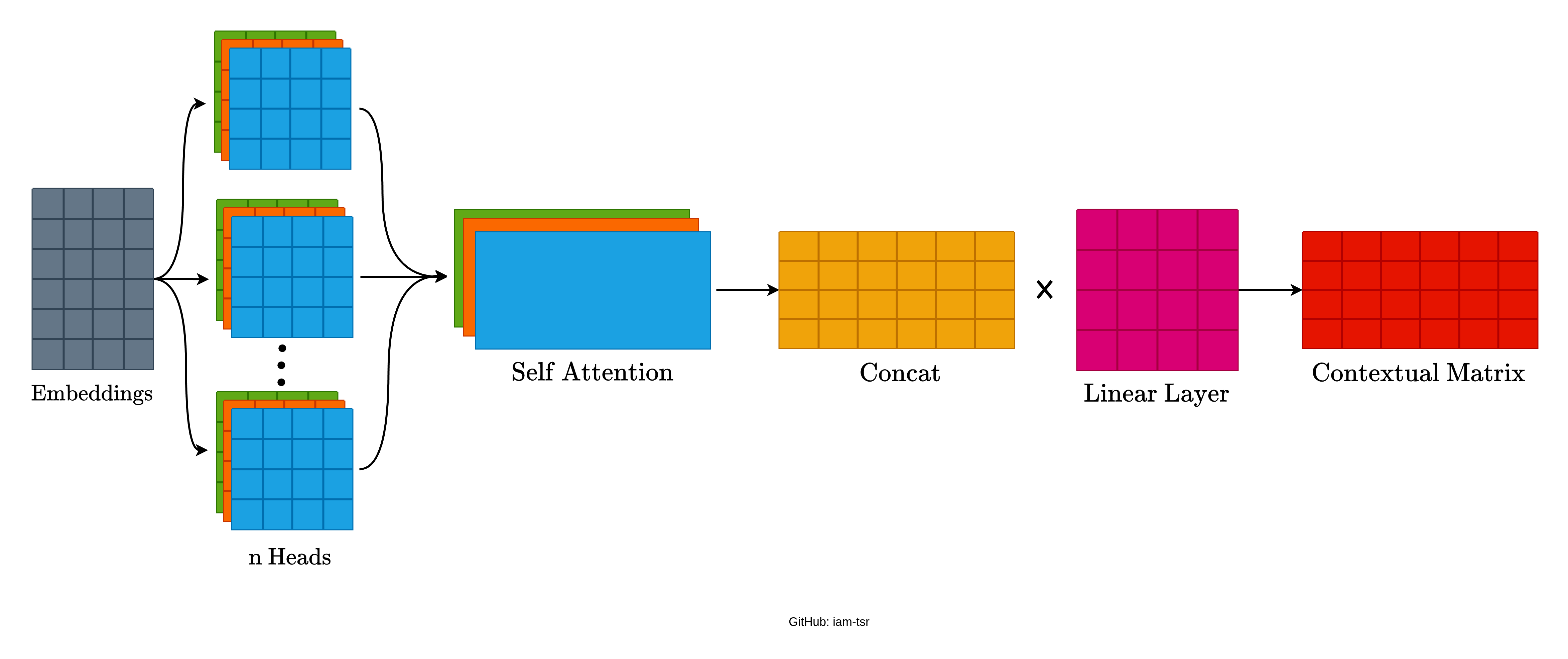
Of course, running multiple attention mechanisms with the full hidden dimension would be computationally expensive. Instead of giving every head the entire embedding, the model splits the hidden dimension evenly across all attention heads.

For example, in BERT Base:

• Hidden dimension = $768$
• Number of attention heads = $12$

So each head operates on vectors of size:

$$\frac{\text{Hidden dimension}}{\text{Number of heads}}=\frac{768}{12}=64$$

Each attention head therefore receives tensors with the shape:

$$\begin{gathered} [1,6,64] \\ \text{instead of,}[1,6,768] \end{gathered}$$

Each head independently computes its own Query, Key, Value, and Scaled Dot-Product Attention. Once all heads finish their computation, their outputs are concatenated along the last dimension.

Since each of the $12$ heads produces a $64-dimensional$ output, concatenating them reconstructs the original hidden size:

$$[12\times 64=768]$$

This produces the contextual embeddings, whose shape becomes:

$$[1,6,768]$$

FAQ

Q. Why do we still multiply the concatenated output by a linear layer?

At first glance, the concatenated output already has the desired hidden size of $768$, so it might seem unnecessary to apply another linear transformation. However, simply concatenating the heads doesn't actually combine the information they have learned.
Think of the concatenated matrix as twelve separate feature groups placed side by side. The first $64$ columns come entirely from Head $1$, the next 64 from Head $2$, and so on. Although they're now stored in one matrix, each head's information is still isolated.
To allow these different perspectives to interact, the Transformer applies one final learnable projection matrix, commonly denoted as $(W^O)$. This output projection mixes information from all attention heads, enabling the model to combine the patterns discovered by each head into a single unified representation.
Mathematically, the operation is: $[1,6,768]$.
This final projection produces the output that is passed to the next layer of the Transformer.

Applying Bi-directional masking

Now that we've seen how the encoder builds contextual representations, let's look at one of the ideas that made models like BERT so effective: bidirectional masking.

It's important to distinguish between the attention mechanism and the training objective. An encoder always uses bidirectional self-attention, meaning every token can attend to both the words before it and the words after it. However, randomly masking tokens is only used during pretraining, not during every task.

For tasks such as text classification, sentiment analysis, or spam detection, the model receives the complete input sentence without masking. Since the objective is simply to classify the text using all available context, there is no need to hide any words.

During Masked Language Modeling (MLM) pretraining, however, the process is different. A small percentage of tokens are randomly replaced with a special [MASK] token, and the model is trained to predict the missing word by looking at the surrounding context from both directions.

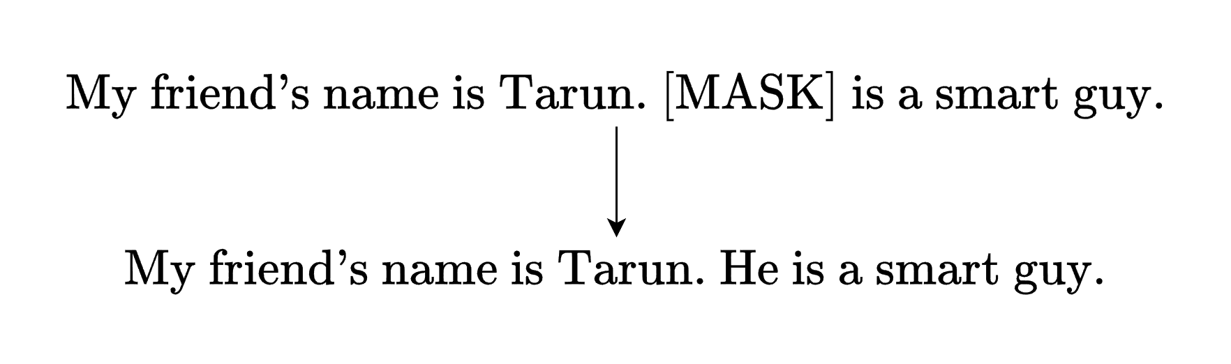
Here, the model uses the words before and after the masked position to predict the missing token: $"He"$

This ability to learn from both the left and right context simultaneously is what gives encoder-only Transformers their strong understanding of language.

Feed Forward Network (FFN)

At this point, the attention mechanism has already done its job. Every token now carries information gathered from the rest of the sequence. But the Transformer isn't finished yet. It still needs a way to further process these contextual representations and learn more complex patterns.

That's where the Feed Forward Network (FFN) comes in. Unlike the attention layer, which allows tokens to interact with one another, the FFN processes each token independently. The same neural network is applied to every token in the sequence, expanding its feature space, applying a non-linear transformation, and then projecting it back to the original hidden dimension.

A typical FFN consists of:

• A linear (dense) layer that expands the hidden dimension.
• An activation function that introduces non-linearity.
• A dropout layer for regularization (used during training).
• A second linear (dense) layer that projects the representation back to the original hidden dimension.

For example, in BERT Base, the hidden dimension is first expanded from $768$ to $3072$, transformed by the activation function, and then projected back to $768$ before being passed to the next Transformer block.

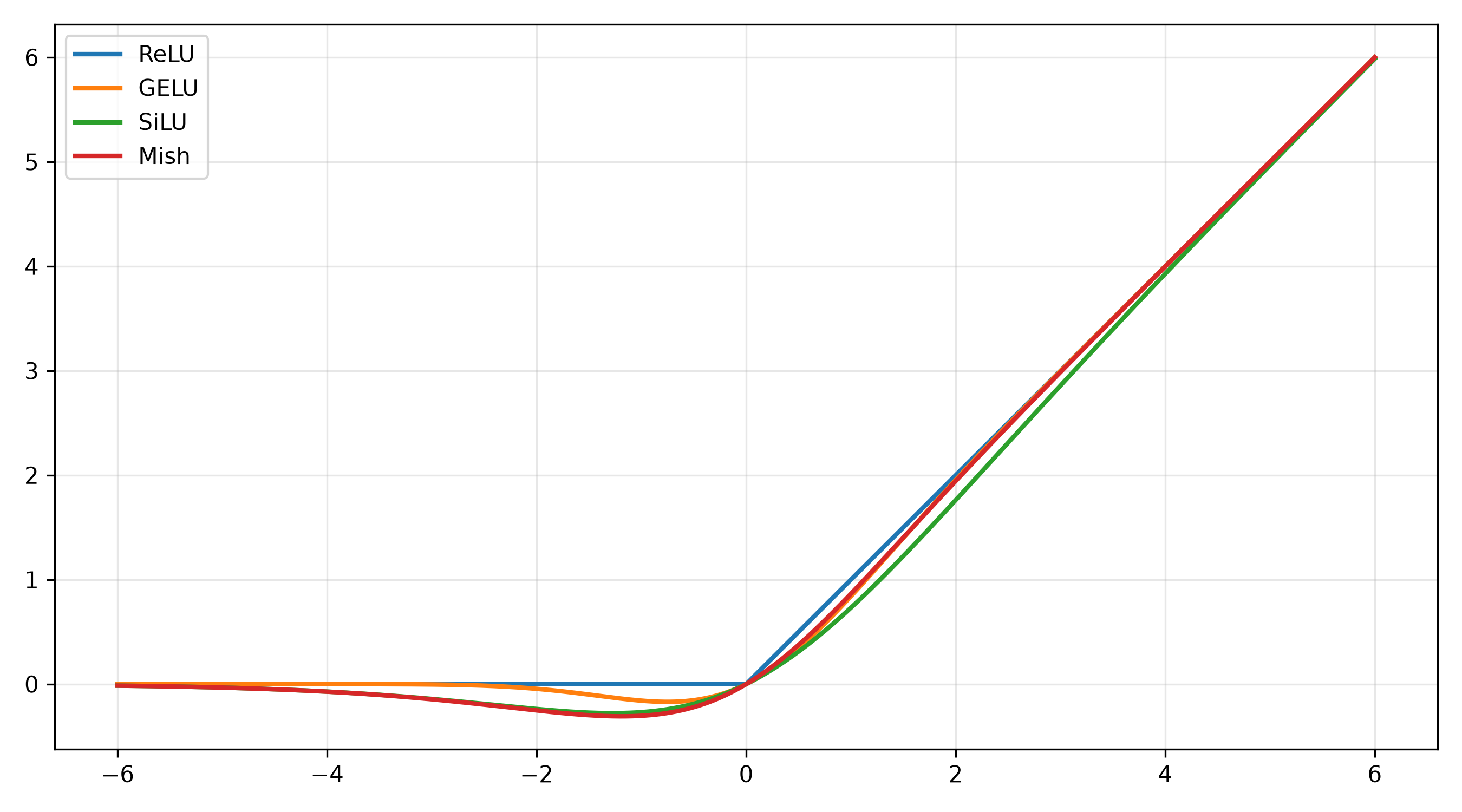
Popular activation function, also used in first transformer architecture are:

ReLU (Rectified Linear Unit)

The original Attention Is All You Need paper used ReLU, making it the first activation function used in Transformer architectures. Its popularity comes from one simple idea: keep positive values unchanged while setting all negative values to zero.

$$\mathrm{Relu}(x)=\max (0,x)$$

This simple operation makes ReLU extremely fast to compute and helps alleviate the vanishing gradient problem that plagued earlier activation functions like Sigmoid and Tanh. Because of its efficiency, ReLU became the default choice for deep neural networks for many years.

The downside is that ReLU completely discards negative values. Once a neuron consistently produces negative outputs, it may stop updating altogether—a phenomenon known as the dying ReLU problem. This limitation motivated researchers to develop smoother activation functions, many of which are now widely used in modern Transformer models.

GELU (Gaussian Error Linear Unit):

As Transformer architectures evolved, researchers found that GELU often produced better results than ReLU. Instead of making a hard decision between keeping or discarding an activation, GELU smoothly scales the input according to its value. Small negative values are only partially suppressed, while larger positive values pass through almost unchanged.

$$\mathrm{GELU}(x)=x\cdot \Phi (x)$$

where $\Phi (x)$ is the cumulative distribution function (CDF) of the standard normal distribution.
Since computing the exact CDF is relatively expensive, implementations usually use one of the following approximations.

• TanH approximation

  $$\text{GELU}(x)\approx 0.5x\left(1+\tanh \left(\sqrt{\frac{2}{\pi }}\left(x+0.044715x^3\right)\right)\right)$$

• Sigmoid approximation

  $$\text{GELU}(x)\approx x\cdot \sigma (1.702x)$$

Today, GELU is the standard activation function in many Transformer models, including BERT, GPT-2, GPT-3, and Vision Transformers (ViT).

SiLU (Sigmoid Linear Unit) / Swish:

Another popular activation function is SiLU, also known as Swish. Instead of abruptly zeroing out negative values like ReLU, Swish applies a smooth gating mechanism that lets both positive and small negative values contribute to learning.

$$f(x)=x\cdot \sigma (\beta x)=\frac{x}{1+e^{-\beta x}}$$

Google Brain introduced Swish in 2017 after discovering it through automated neural architecture search, although similar formulations had appeared independently before.

Its smooth and non-monotonic shape often leads to better optimization and gradient flow in very deep networks. Today, SiLU is widely used in modern architectures such as EfficientNet, while its gated variant, SwiGLU, powers several recent large language models, including Llama 3, Mistral, and Gemma.

Mish:

Mish is another smooth, self-gated activation function introduced by Diganta Misra in 2019. Like Swish, it allows small negative values to pass through instead of discarding them completely, resulting in a smoother optimization landscape.

$$\text{Mish}(x)=x\cdot \tanh (\text{softplus}(x))=x\cdot \tanh (\ln (1+e^x))$$

Mish demonstrated strong performance in several computer vision benchmarks and became well known through models such as YOLOv4. However, unlike GELU or SwiGLU, it has seen relatively limited adoption in large language models.

Normalization

By now, I'm assuming you're already familiar with what normalization is and why it's such an important part of training deep neural networks. If these concepts are new to you, don't worry—you can still follow along, but I recommend taking a quick look at them first since we'll build on that knowledge here.

Before we dive into the different normalization techniques used in Transformers, there's one more preprocessing concept we need to cover: Padding and Truncation.

Throughout Part 1 of Attention Is Good, we worked with a single sentence to keep the explanations simple and focused. That made it easier to understand tokenization, embeddings, and attention without worrying about batches of different-sized inputs.

Now it's time to level things up. Real-world models rarely process one sentence at a time. Instead, they work on batches of sentences, and those sentences almost never have the same length. To handle this efficiently, Transformers rely on padding and truncation before the data is passed into the model.

We've already built the foundation, so this next step should feel like a natural extension rather than something entirely new.

Padding:

Up until now, we've been working with a single sentence at a time, so every input naturally had the same length. But that's not how Transformers are trained in practice.

During training, we usually process multiple sentences together as a batch. The problem is that natural language is messy—some sentences are short, while others are much longer.

For example:

• $S_1=\text{"Karna was the great warrior"}(\text{5 tokens})$
• $S_2=\text{"Karna was the son of Surya Dev"}(\text{7 tokens})$

After converting these sentences into embeddings with a hidden size of 768, their shapes become: $S_1=[5,768]$ and $S_2=[7,768]$.

These tensors cannot simply be stacked into a single batch because their sequence lengths differ. Deep learning frameworks expect every sequence in a batch to have the same shape.

To solve this problem, we extend the shorter sentence by appending a special $[PAD]$ token until its length matches the longest sequence in the batch.

For example:

• $S_1=\text{"Karna was the great warrior [PAD] [PAD]"}(\text{7 tokens})$
• $S_2=\text{"Karna was the son of Surya Dev"}(\text{7 tokens})$

Now both sequences have the same length, allowing them to be stacked into a single tensor and processed efficiently in parallel.

You might wonder what happens to these padding tokens during training. Although they are assigned an embedding like any other token, the model is also given an attention mask that marks every padding position. During self-attention, these masked positions are ignored, ensuring that the padding contributes nothing to the final contextual representations.

Truncation:

Padding helps us handle sentences that are shorter than the longest sequence in a batch. But what about sentences that are too long?

Every Transformer model has a maximum sequence length that it can process. For example, the original BERT model supports up to 512 tokens. If an input exceeds this limit, the model cannot process the entire sequence as-is.

That's where truncation comes in.

During preprocessing, any tokens beyond the maximum sequence length are simply removed, leaving only the portion of the text that fits within the model's limit. The discarded tokens are not seen by the model and therefore cannot influence its predictions.

Before we move on to normalization, we'll need one small piece of mathematical notation that appears throughout neural networks.

For a single neuron, the output is computed as:

$$y={\mathbf{x}}^{\top }\mathbf{W}+b$$

This calculates output for a single feature. But in text, we handle multiple features (tokens) at once:

where:

• $(\mathbf{x})$ is the input vector,
• $(\mathbf{W})$ is the weight vector,
• $(b)$ is the bias term.

Writing the same equation as a summation gives:

$$y=\sum _{i=1}^n{W}_i{x}_i+b$$

Here, each input feature is multiplied by its corresponding weight, the results are summed together, and finally the bias is added.

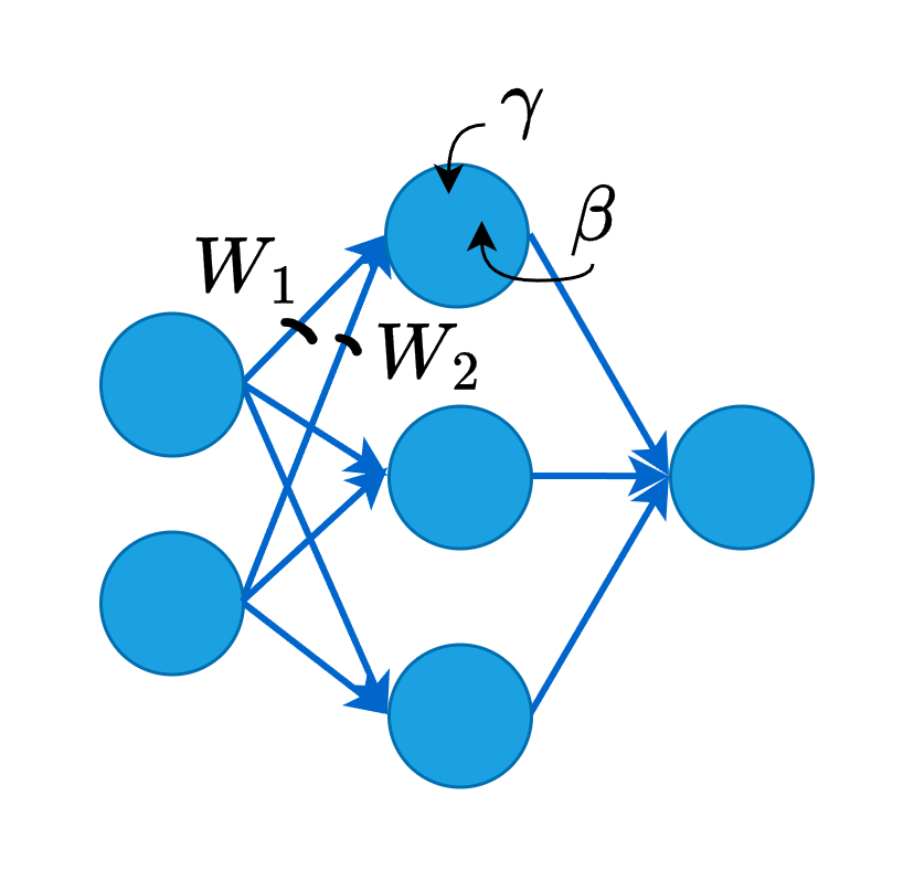
We'll use this equation repeatedly in the upcoming sections when we discuss normalization and the Feed Forward Network, so it's worth keeping it in mind.

There are two widely known normalization techniques used in deep learning. Although both aim to stabilize training and improve convergence, they normalize data in very different ways.

Batch Normalization

Batch Normalization was a breakthrough for convolutional neural networks, but it is rarely used in Transformer architectures. Instead, modern Transformers almost universally rely on Layer Normalization.

Let's first understand how Batch Normalization works.

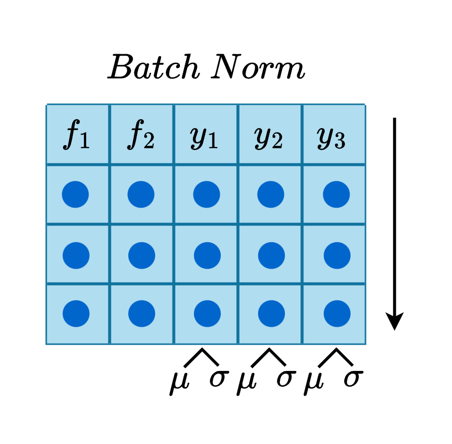
Suppose we have two input features, $f_1$ and $f_2$, feeding into a neural network. Each neuron in the hidden layer computes its output using the familiar perceptron equation:

$$y=\sum _{i=1}^n{W}_i{x}_i+b$$

This produces the activations $y_1$, $y_2$, and $y_3$. Batch Normalization then computes the mean $(\mu )$ and standard deviation $(\sigma )$ of these activations across the entire mini-batch before normalizing them.

The normalized output is given by:

$$z=\gamma \left(\frac{x-\mu }{\sqrt{{\sigma }^2+ϵ}}\right)+\beta$$

where:

• $(\gamma )$ is a learnable scaling parameter (initialized to 1).
• $(\beta )$ is a learnable bias parameter (initialized to 0).
• $(ϵ)$ is a very small constant added for numerical stability.

Although Batch Normalization works exceptionally well for CNNs, it is less suitable for Transformers because it depends on batch-wide statistics. In natural language processing, batches often contain sequences of different lengths, requiring padding. While attention masks prevent the model from attending to padding tokens, Batch Normalization still computes statistics over activations within the batch, making it less robust for variable-length sequential data. Layer Normalization avoids this dependency altogether.

Layer Normalization

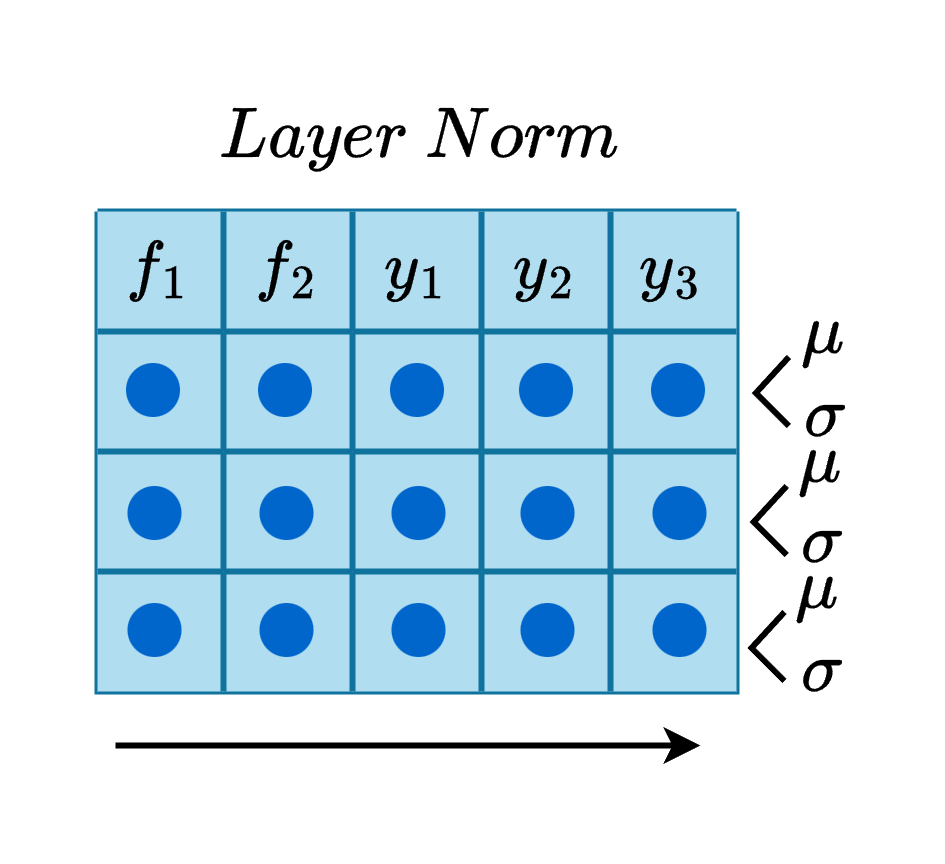
Instead of normalizing across the entire batch, Layer Normalization normalizes each token independently across its feature dimensions.

In other words, if a token is represented by a $768$-dimensional embedding, Layer Normalization computes the mean and variance using only those $768$ values. Every token performs this computation independently, regardless of what other tokens or other sentences exist in the batch.

Because Layer Normalization does not depend on batch statistics, it naturally handles varying batch sizes, variable-length sequences, and padded inputs. This is one of the main reasons it became the standard normalization technique in almost every modern Transformer architecture, including BERT, GPT, ViT, Llama, Gemma, and Mistral.

If you'd like a deeper mathematical explanation of Layer Normalization, you can refer to Campus X.

Implementaion of Layer Normalization

Once Layer Normalization became the standard choice for Transformers, researchers began experimenting with where it should be placed inside each Transformer block. Surprisingly, this seemingly small design choice has a significant impact on training stability and model performance.

Over the years, three notable designs have emerged.

Post LN:

The original Attention Is All You Need paper introduced the Post-LN architecture. In this design, Layer Normalization is applied after the residual (skip) connection in both the Multi-Head Attention (MHA) block and the Feed Forward Network (FFN).

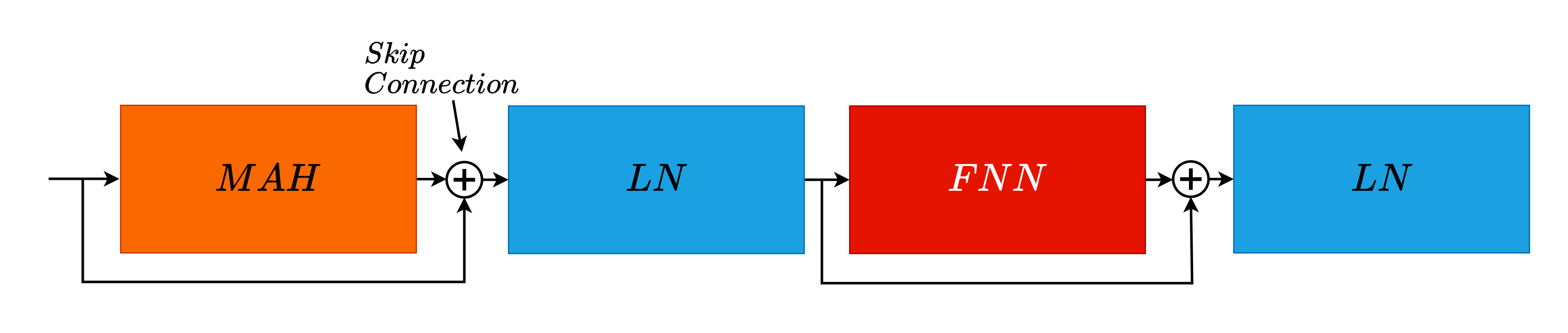
The $(\oplus )$ symbol represents a skip connection (also called a residual connection). Instead of passing information through only the current layer, the input is added directly to the layer's output before normalization.

These skip connections provide a shorter path for gradients during backpropagation, making it easier for information to flow through the network and helping mitigate the vanishing gradient problem.

Although Post-LN works well for relatively shallow Transformers, it becomes increasingly difficult to optimize as models grow deeper. Researchers observed that deep Post-LN models are more prone to gradient instability, making training less reliable.

Pre LN:

To address these optimization challenges, researchers proposed Pre-LN, where Layer Normalization is moved before the Multi-Head Attention and Feed Forward Network.

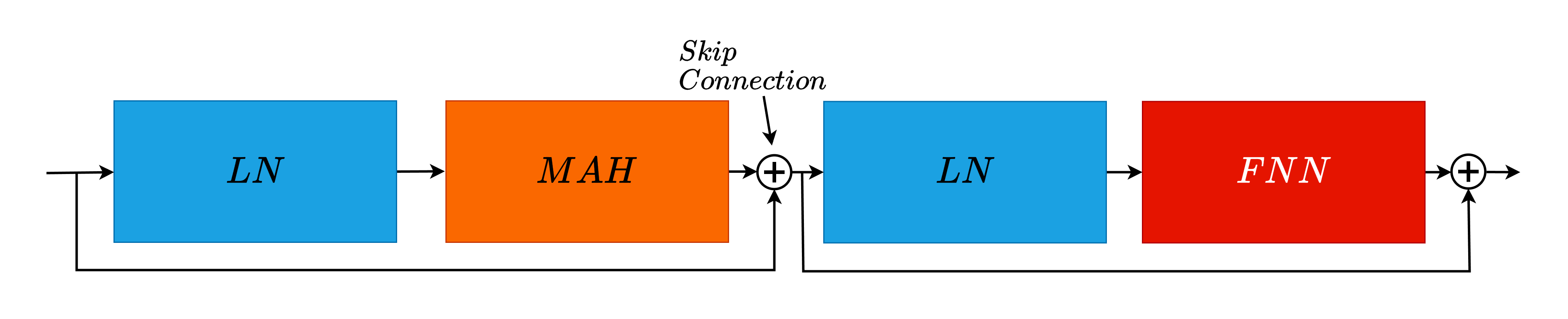
This seemingly simple rearrangement dramatically improves gradient flow, allowing much deeper Transformer models to train more stably. Because of this advantage, Pre-LN has become a popular choice in many modern architectures.

However, later research found that very deep Pre-LN models can suffer from representation collapse, where hidden representations across layers become increasingly similar, reducing the diversity of learned features. While the model still trains successfully, this phenomenon can limit representational quality in extremely deep networks.

ResiDual:

More recently, researchers proposed ResiDual, an architecture designed to combine the strengths of both Post-LN and Pre-LN.

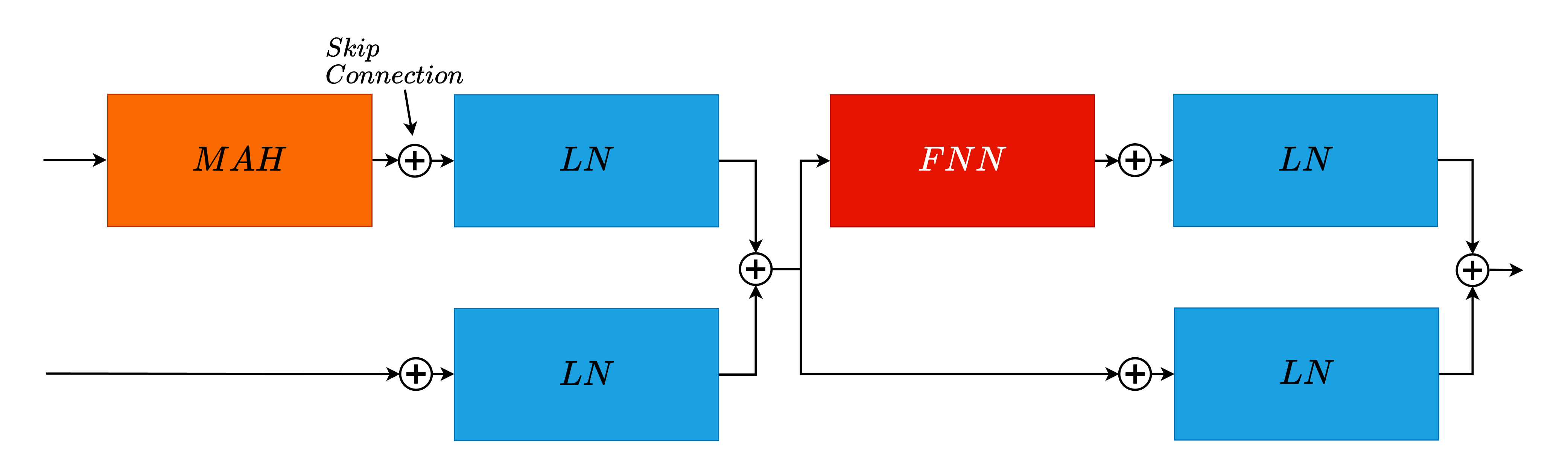
The illustration shown here has not been independently verified, as I do not have access to the resources or faculty available at leading academic institutions. This illustration is adapted from the YouTube video by Machine Learning Studio.

If you have the opportunity to discuss it with professors or experts at your institution, I'd appreciate hearing whether they validate its accuracy.

Instead of choosing between optimization stability and representational quality, ResiDual introduces dual residual connections that aim to preserve healthy gradient flow while also maintaining richer intermediate representations.

Although it is not yet the standard Transformer design, ResiDual demonstrates that careful placement of normalization and residual connections can address many of the weaknesses observed in earlier Layer Normalization strategies.

Classification Head

After passing through multiple Transformer layers, every token in the sequence has been enriched with contextual information from the entire sentence. At this stage, the encoder has done its job—it has learned meaningful representations. The only thing left is to convert those representations into predictions.

This is the role of the Classification Head.

The classification head is typically a simple linear layer, although some architectures replace it with a small Multi-Layer Perceptron (MLP) for additional learning capacity.

Suppose the encoder produces an output tensor with the shape: $[\text{batch size},\text{sequence length},\text{hidden size}]$

For sentence-level classification tasks, we first need a single vector that represents the entire sequence. In BERT, this is usually the embedding corresponding to the special $[CLS]$ token, giving a tensor of shape: $[\text{batch size},\text{hidden size}]$

Some encoder models instead use techniques such as mean pooling or max pooling over all token representations, but the goal is the same: obtain one vector that summarizes the entire input.

The classification head then projects this vector into the desired number of output classes:

$$[\text{batch size},\text{hidden size}]\to [\text{batch size},\text{number of classes}]$$

The output of this projection is called logits.

The choice of the final activation depends on the task:

• Softmax for multi-class classification, where each example belongs to exactly one class.
• Sigmoid for multi-label classification, where an example can belong to multiple classes simultaneously.

For example, in a sentiment analysis task, the encoder first builds a contextual understanding of the entire sentence. The classification head then converts that representation into logits, which are transformed into probabilities for classes such as positive, neutral, and negative.

---

Next, we'll explore the decoder-only architecture of the Transformer. Until then, keep learning, keep growing, and continue shaping yourself!